Excel is one of the most used programs by professionals. Microsoft’s spreadsheet editor has features that go far beyond formulas: it allows you to create visual panels, perform data searches, Excel functions create graphics for presentations, among countless other features. The tools are available in their entirety for the desktop — whether in Windows or macOS — and, to a large extent, also in Android and iPhone (iOS) mobile apps.
The spreadsheet program in the Office suite concentrates several options that help in the day-to-day — professional and personal — of its users. MKTPlace has separated a list with six useful functions for those who work with the editor.
1. Dashboards
A dashboard is a visual dashboard that shows all the important information about a business or process. It helps organize data and metrics that will be taken into account when making decisions. This ability is interesting for many professions, but it is especially used by IT professionals and in business management.
In Excel, the first step to create a dashboard is to build a spreadsheet with the data you want to display in the dashboard. Then you need to select it, go to the “Insert” menu and select “Pivot Table”.
Select two fields and create the pivot table, repeating the process with different fields to form multiple tables. The next step is to build dynamic charts with the assembled tables. At the end, you’ll have a dashboard full of information organized in a much more intuitive way than in the original spreadsheet.
2. Graphics
Graphing is another visual solution for organizing data. They are used by a huge amount of professionals such as managers, accountants, IT workers, human resources and others. The function is also very useful for students and teachers, as well as anyone who wants to give presentations.
Excel has a huge variety of chart types, such as pie, bar, line, column, area, radar, among others. To generate a graph, just select the table with the database, click on the “Insert” menu and select the preferred model. Each type can even be customized with colors, styles, fonts, alignments and design to the user’s taste.
3. NPV
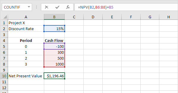
Excel functions allows you to calculate the Net Present Value (NPV), an account used by investors to find the real gain of an application. The calculation is necessary for both individual investors and entrepreneurs who wish to increase their company’s equity.
Microsoft’s spreadsheet editor has the VPL function. The formula is “=vpl(rate;value)”, without quotes, and must be typed in a blank cell. If there is more than one period, it must be added in sequence.

4. Pivot table
Excel pivot tables synthesize data from very large tables, making it easy to analyze information. They are automatically updated when the values in the original table are changed, keeping the information always correct. These characteristics make the resource interesting for positions that deal with a large volume of information, such as personnel department managers, marketers, developers, etc.
After selecting a simple table, go to “Insert” and choose “Pivot Table”. As described in creating dashboards, you can create multiple pivot tables using different fields from the same original table. They can be entered in the same spreadsheet as the original or in a new one — the automatic update will work just as well.
5. Conditional formatting
Conditional formatting is for highlighting cells based on certain values or parameters. For example, you want to quickly see which months you spent more than US$1000 in the supermarket. To do this, just take the household budget spreadsheet and apply conditional formatting so that Excel will redden the cells larger than this amount.
The feature, which can be used by virtually all professionals who work behind their computer screen, is located within the “Home Page”. Select the table and click on the menu to view the tool. Excel provides a shortcut to the most popular templates, but you can edit conditional formatting by going to “More rules” to create your own standards.
6. PROCV
Excel’s VLOOKUP function lets you find data in rows of a table or a range. It performs a vertical search — that is, along a column — based on a given value and offering in response other data from the corresponding row, where the searched value was found. In this way, it links different tables, avoiding duplication of data and typing errors.
Its formula is “=VLOOKUP(search_value;table_array;column_index_num;[search_range])”, without quotes. In this string, “search_value” is what you want to find; “table_array” is the interval where the function will perform the search; “column_index_num” is the number of the column where the answer will be displayed; and “search_range”, optional padding, allows the user to define whether they want VLOOKUP to find an exact or approximate match. Yes, Excel functions are so usefull!
